Tutorial: model fitting with correlated noise¶

In this example, we’re going to simulate a common data analysis situation where our dataset exhibits unknown correlations in the noise. When taking data, it is often possible to estimate the independent measurement uncertainty on a single point (due to, for example, Poisson counting statistics) but there are often residual systematics that correlate data points. The effect of this correlated noise can often be hard to estimate but ignoring it can introduce substantial biases into your inferences. In the following sections, we will consider a synthetic dataset with correlated noise and a simple non-linear model. We will start by fitting the model assuming that the noise is uncorrelated and then improve on this model by modeling the covariance structure in the data using a Gaussian process.

All the code used in this tutorial is available here.

A Simple Mean Model¶

The model that we’ll fit in this demo is a single Gaussian feature with three parameters: amplitude \(\alpha\), location \(\ell\), and width \(\sigma^2\). I’ve chosen this model because is is the simplest non-linear model that I could think of, and it is qualitatively similar to a few problems in astronomy (fitting spectral features, measuring transit times, etc.).

Simulated Dataset¶

I simulated a dataset of 50 points with known correlated noise. In fact, this example is somewhat artificial since the data were drawn from a Gaussian process but in everything that follows, we’ll use a different kernel function for our inferences in an attempt to make the situation slightly more realistic. A known white variance was also added to each data point and the resulting dataset is:

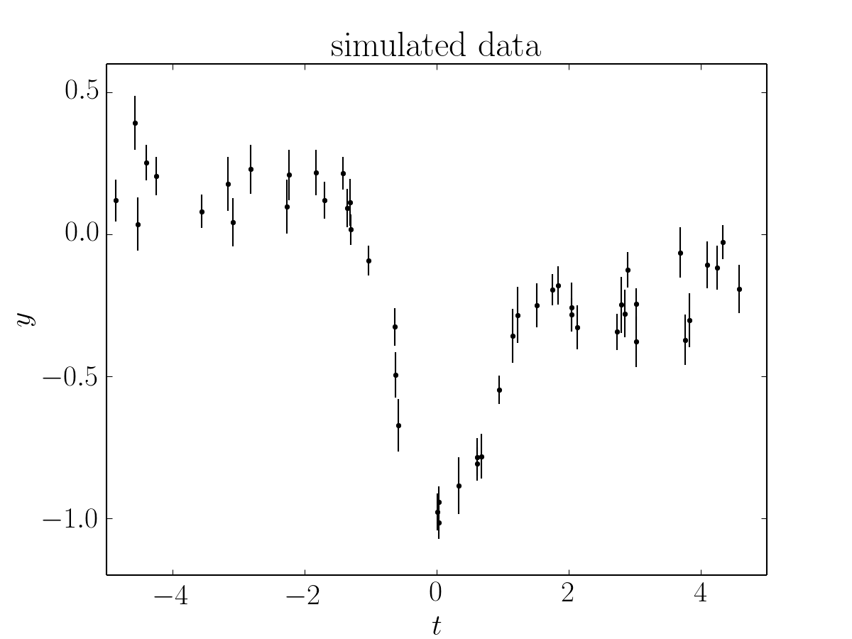
The true model parameters used to simulate this dataset are:

\[\alpha = -1\quad, \quad\quad \ell = 0.1\quad, \quad\quad \sigma^2 = 0.4\quad.\]

Assuming White Noise¶

Let’s start by doing the standard thing and assuming that the noise is uncorrelated. In this case, the ln-likelihood function of the data \(\{y_n\}\) given the parameters \(\theta\) is

\[\ln p(\{y_n\}\,|\,\{t_n\},\,\{\sigma_n^2\},\,\theta) = -\frac{1}{2}\,\sum_{n=1}^N \frac{[y_n - f_\theta(t_n)]^2}{\sigma_n^2} + A\]

where \(A\) doesn’t depend on \(\theta\) so it is irrelevant for our purposes and \(f_\theta(t)\) is our model function.

It is clear that there is some sort of systematic trend in the data and we don’t want to ignore that so we’ll simultaneously model a linear trend and the Gaussian feature described in the previous section. Therefore, our model is

\[f_\theta (t) = m\,t + b + \alpha\,\exp\left(-\frac{[t-\ell]^2}{2\,\sigma^2} \right)\]

where \(\theta\) is the 5-dimensional parameter vector

\[\theta = \{ m,\,b,\,\alpha,\,\ell,\,\sigma^2 \} \quad.\]

The following code snippet is a simple implementation of this model in Python

import numpy as np

def model1(params, t):
    m, b, amp, loc, sig2 = params
    return m*t + b + amp * np.exp(-0.5 * (t - loc) ** 2 / sig2)

def lnlike1(p, t, y, yerr):
    return -0.5 * np.sum(((y - model1(p, t))/yerr) ** 2)

To fit this model using MCMC (using emcee), we need to first choose priors—in this case we’ll just use a simple uniform prior on each parameter—and then combine these with our likelihood function to compute the ln-probability (up to a normalization constant). In code, this will be:

def lnprior1(p):
    m, b, amp, loc, sig2 = p
    if (-10 < m < 10 and  -10 < b < 10 and -10 < amp < 10 and
            -5 < loc < 5 and 0 < sig2 < 3):
        return 0.0
    return -np.inf

def lnprob1(p, x, y, yerr):
    lp = lnprior1(p)
    return lp + lnlike1(p, x, y, yerr) if np.isfinite(lp) else -np.inf

Now that we have our model implemented, we’ll initialize the walkers and run both a burn-in and production chain:

# We'll assume that the data are stored in a tuple:
#    data = (t, y, yerr)

import emcee

initial = np.array([0, 0, -1.0, 0.1, 0.4])
ndim = len(initial)
p0 = [np.array(initial) + 1e-8 * np.random.randn(ndim)
      for i in xrange(nwalkers)]
sampler = emcee.EnsembleSampler(nwalkers, ndim, lnprob1, args=data)

print("Running burn-in...")
p0, _, _ = sampler.run_mcmc(p0, 500)
sampler.reset()

print("Running production...")
sampler.run_mcmc(p0, 1000)

After running the chain, we can plot the results using the flatchain property of the sampler. It is often useful to plot the results on top of the data as well. To do this, we can over plot 24 posterior samples on top of the data:

import matplotlib.pyplot as pl

# Plot the data.
pl.errorbar(t, y, yerr=yerr, fmt=".k", capsize=0)

# The positions where the prediction should be computed.
x = np.linspace(-5, 5, 500)

# Plot 24 posterior samples.
samples = sampler.flatchain
for s in samples[np.random.randint(len(samples), size=24)]:
    pl.plot(x, model1(s, x), color="#4682b4", alpha=0.3)

Running this code should make a figure like:

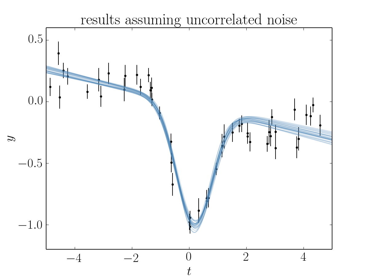
In this figure, the data are shown as black points with error bars and the posterior samples are shown as translucent blue lines. These results seem, at face value, pretty satisfying. But, since we know the true model parameters that were used to simulate the data, we can assess our original assumption of uncorrelated noise. To do this, we’ll plot all the projections of our posterior samples using triangle.py and over plot the true values:

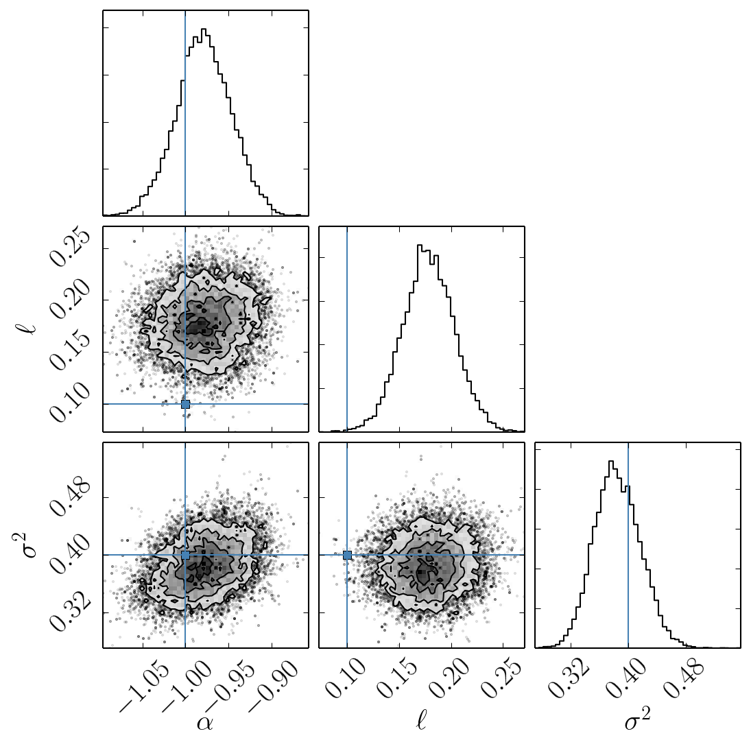
In this figure, the blue lines are the true values used to simulate the data and the black contours and histograms show the posterior constraints. The constraints on the amplitude \(\alpha\) and the width \(\sigma^2\) are consistent with the truth but the location of the feature \(\ell\) is almost completely inconsistent with the truth! This would matter a lot if we were trying to precisely measure radial velocities or transit times.

Modeling the Noise¶

Note

A full discussion of the theory of Gaussian processes is beyond the scope of this demo—you should probably check out Rasmussen & Williams (2006)—but I’ll try to give a quick qualitative motivation for our model.

In this section, instead of assuming that the noise is white, we’ll generalize the likelihood function to include covariances between data points. To do this, let’s start by re-writing the likelihood function from the previous section as a matrix equation (if you squint, you’ll be able to work out that we haven’t changed it at all):

\[\ln p(\{y_n\}\,|\,\{t_n\},\,\{\sigma_n^2\},\,\theta) = -\frac{1}{2}\,\boldsymbol{r}^\mathrm{T}\,K^{-1}\,\boldsymbol{r} -\frac{1}{2}\,\ln\det K - \frac{N}{2}\,\ln 2\pi\]

where

\[\begin{split}\boldsymbol{r} = \left ( \begin{array}{c} y_1 - f_\theta(t_1) \\ y_2 - f_\theta(t_2) \\ \vdots \\ y_N - f_\theta(t_N) \\ \end{array}\right)\end{split}\]

is the residual vector and

\[\begin{split}K = \left ( \begin{array}{cccc} \sigma_1^2 & 0 & & 0 \\ 0 & \sigma_2^2 & & 0 \\ & & \ddots & \\ 0 & 0 & & \sigma_N^2 \\ \end{array}\right)\end{split}\]

is the \(N \times N\) data covariance matrix (where \(N\) is the number of data points).

The fact that \(K\) is diagonal is the result of our earlier assumption that the noise was white. If we want to relax this assumption, we just need to start populating the off-diagonal elements of this covariance matrix. If we wanted to make every off-diagonal element of the matrix a free parameter, there would be too many parameters to actually do any inference. Instead, we can simply model the elements of this array as

\[K_{ij} = \sigma_i^2\,\delta_{ij} + k(t_i,\,t_j)\]

where \(\delta_{ij}\) is the Kronecker_delta and \(k(\cdot,\,\cdot)\) is a covariance function that we get to choose. Chapter 4 of Rasmussen & Williams discusses various choices for \(k\) but for this demo, we’ll just use the Matérn-3/2 function:

\[k(r) = a^2 \, \left( 1+\frac{\sqrt{3}\,r}{\tau} \right)\, \exp \left (-\frac{\sqrt{3}\,r}{\tau} \right )\]

where \(r = |t_i - t_j|\), and \(a^2\) and \(\tau\) are the parameters of the model.

The Final Fit¶

Now we could go ahead and implement the ln-likelihood function that we came up with in the previous section but that’s what George is for, after all! To implement the model from the previous section using George, we can write the following ln-likelihood function in Python:

import george
from george import kernels

def model2(params, t):
    _, _, amp, loc, sig2 = params
    return amp * np.exp(-0.5 * (t - loc) ** 2 / sig2)

def lnlike2(p, t, y, yerr):
    a, tau = np.exp(p[:2])
    gp = george.GP(a * kernels.Matern32Kernel(tau))
    gp.compute(t, yerr)
    return gp.lnlikelihood(y - model2(p, t))

def lnprior2(p):
    lna, lntau, amp, loc, sig2 = p
    if (-5 < lna < 5 and  -5 < lntau < 5 and -10 < amp < 10 and
            -5 < loc < 5 and 0 < sig2 < 3):
        return 0.0
    return -np.inf

def lnprob2(p, x, y, yerr):
    lp = lnprior2(p)
    return lp + lnlike2(p, x, y, yerr) if np.isfinite(lp) else -np.inf

As before, let’s run MCMC on this model:

initial = np.array([0, 0, -1.0, 0.1, 0.4])
ndim = len(initial)
p0 = [np.array(initial) + 1e-8 * np.random.randn(ndim)
      for i in xrange(nwalkers)]
sampler = emcee.EnsembleSampler(nwalkers, ndim, lnprob2, args=data)

print("Running first burn-in...")
p = p0[np.argmax(lnp)]
sampler.reset()

# Re-sample the walkers near the best walker from the previous burn-in.
p0 = [p + 1e-8 * np.random.randn(ndim) for i in xrange(nwalkers)]
p0, _, _ = sampler.run_mcmc(p0, 250)

print("Running second burn-in...")
p0, _, _ = sampler.run_mcmc(p0, 250)
sampler.reset()

print("Running production...")
sampler.run_mcmc(p0, 1000)

You’ll notice that this time I’ve run two burn-in phases where each one is half the length of the burn-in from the previous example. Before the second burn-in, I re-sample the positions of the walkers in a tiny ball around the position of the best walker in the previous run. I found that this re-sampling step was useful because otherwise some of the walkers started in a bad part of parameter space and took a while to converge to something reasonable.

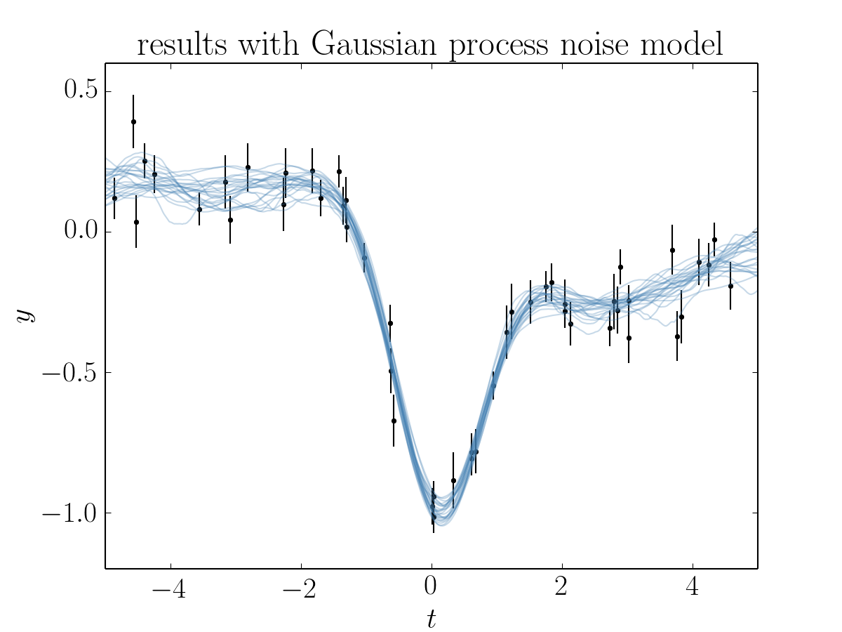
The plotting code for the results for this model is similar to the code in the previous section. First, we can plot the posterior samples on top of the data:

# Plot the data.
pl.errorbar(t, y, yerr=yerr, fmt=".k", capsize=0)

# The positions where the prediction should be computed.
x = np.linspace(-5, 5, 500)

# Plot 24 posterior samples.
samples = sampler.flatchain
for s in samples[np.random.randint(len(samples), size=24)]:
    # Set up the GP for this sample.
    a, tau = np.exp(s[:2])
    gp = george.GP(a * kernels.Matern32Kernel(tau))
    gp.compute(t, yerr)

    # Compute the prediction conditioned on the observations and plot it.
    m = gp.sample_conditional(y - model2(s, t), x) + model(s, x)
    pl.plot(x, m, color="#4682b4", alpha=0.3)

This code should produce a figure like:

The code for the corner plot is identical to the previous one. Running that should give the following marginalized constraints:

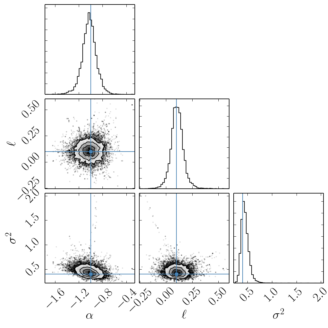
It is clear from this figure that the constraints obtained when modeling the noise are less precise (the error bars are larger) but more accurate (less biased).